Following up on this post, estimating the consumption function
Consider the canonical consumption-income relationship discussed in macro textbooks. For pedagogical reasons, the relationship is often stated as:
(1) C = c0 + c1 Yd
Where C is real consumption and Yd is real disposable income. Figure 1 depicts the relationship over the 1967-2015Q2 period.
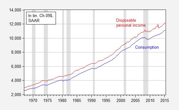
Figure 1: Consumption (blue) and disposable personal income (red), in billions of Ch.2009$, SAAR. NBER defined recession dates shaded gray. Source: BEA, 2015Q2 advance release, and NBER.
Now consider the corresponding figure, in logs (denoted by lowercase letters).
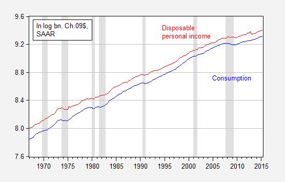
Figure 2: Log consumption (blue) and log disposable personal income (red), in billions of Ch.2009$, SAAR. NBER defined recession dates shaded gray. Source: BEA, 2015Q2 advance release, and NBER.
It does seem hard to choose one over the other merely by looking. Reader Mike V writes:
I just think you lose a lot of people by using logs for every. graph.
Which one is the better way to characterize the relationship? I will note that one distinct advantage of the logged version is that one can immediately see at what times consumption growth rates slow — and that is in Figure 2. Looking at Figure 1, one might have thought consumption growth rates were higher in the 2000’s (up to 2007) than the 1990’s. But the logged values in Figure 2 allows one to see past that illusion (constant growth rates are a straight line when examining logged values; see Jim’s post for more). While not a definitive reason to prefer logs, it is useful for quick data assessment.
At first glance, estimating each by way of OLS does not allow much to distinguish between the two representations. In levels:
(2) C = -336.7 + 0.945Yd
R2 = 0.999, SER = 93.26, Nobs = 194, DW = 0.56. Bold Face indicates significance at 5% msl using HAC standard errors.
In logs:
(3) c = -0.651 + 1.061yd
R2 = 0.999, SER = 0.014, Nobs = 194, DW = 0.48. Bold Face indicates significance at 5% msl using HAC standard errors.
Clearly, neither specification is adequate, but is one to be preferred to another? Theory does not provide guidance, as the linear consumption function is typically used for convenience.
One factor one can use to inform a choice is heteroscedasticity, the characteristic wherein the variance of the errors is not constant. One does not observe the true residuals, but one can examine the squared estimated residuals, and see if there is a systematic pattern between the squared residuals and the right hand side variable. Figure 3 presents the squared residuals from the levels specification, and Figure 4 presents squared residuals from the log specification.
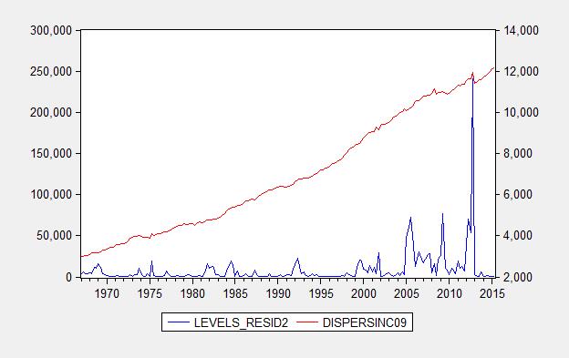
Figure 3: Squared residuals from levels regression (2).
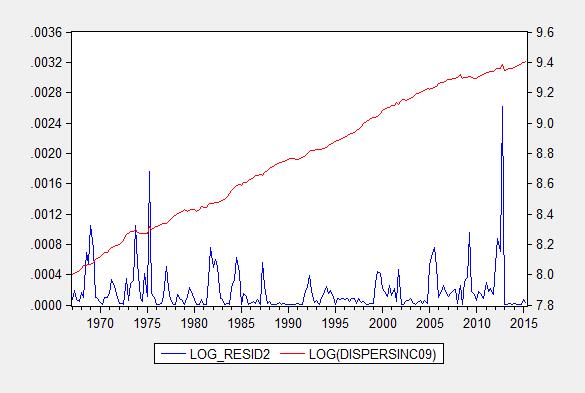
Figure 4: Squared residuals from log levels regression (3).
While in both cases the residuals exhibit a (positive) correlation with the right hand side variable, it is much more pronounced in the levels regression. In other words, the real dollar errors increase systematically with real dollar disposable income, while (log) percent errors increase less strongly with percent increases in real disposable income. This provides one reason to prefer a log specification. By the way, a Jarque-Bera test rejects normality for both residuals, but much more soundly for the levels specification.
Now, the residuals exhibit substantial serial correlation (rule of thumb: possible spurious correlation of integrated series if the R2 > DW). This suggests estimating a cointegrating relationship (see this post) or – if one wants the short run dynamics – an error correction model. The analogs to equations (2) and (3) (after augmenting with household net worth to account for life-cycle effects) are:
(4) ΔCt = 1.900 + 0.027Ct-1 – 0.018Yd,t-1 – 0.0008Wt-1 + lagged first difference terms
R2 = 0.25, SER = 33.55, Nobs = 192, DW = 2.21. Bold Face indicates significance at 5% msl.
In logs:
(5) Δct = 0.014 – 0.017ct-1 + 0.011 yd,t-1 + 0.004wt-1 + lagged first difference terms
R2 = 0.21, SER = 0.006, Nobs = 192, DW = 2.18. Bold Face indicates significance at 5% msl.
In this case, there is no clear advantage to one specification or the other. The levels specification indicates explosive behavior (as the coefficient on the lagged level of the dependent variable is positive; but it’s not statistically significant). Only the lagged differenced variables are statistically significant. In the log specification, the implied behavior is not explosive, given the coefficient on the lagged log level of the dependent variable; actually given the non-significance of the coefficient, there does not appear to be evidence of cointegration (actually, all that we know is that consumption does not seem to revert to re-establish the long run relationship between consumption, income and wealth – it might be that the other two variables do the adjustment, and in fact a Johansen test suggests this is the case).
For a more detailed analysis, disaggregating consumption data, see this post. In that case, logs in conjunction with disaggregation seems to do the trick.
Apart from the question of whether to log or not log there is a more serious problem here.
The assumption here (as in Keynes’s propensity to consume hypothesis and Friedman’s permanent income hypothesis) is that consumption is dependent on income. And for the individual that is indeed so. But for the aggregate economy it is not so, as I have shown in my book Macroeconomics Redefined. Income is a function of consumption and not the other way around.
When there is a financial asset market crash consumers lose a large chunk of their net worth and so curtail their consumption expenditure (because they raise their saving rate in a bid to recoup lost savings). When businesses see this they curtail their output, so aggregate income falls. Consumer expenditure lags this fall in business output by a short period. This is because businesses first cut output but retain their employees because they are not sure whether the fall in demand is long-lived or not.
In the 2008 crash the median household lost 18 years of its net worth. To regain this it would need to double its saving rate for 18 years, other things being equal. That is why recoveries following financial asset crashes are as protracted as they are. As savings are recouped both consumption expenditures and income recover.
That is also apparent from the first graph which shows that consumption expenditures remain stable even when there are sudden rises in disposable income. All such income increases go straight to savings.
In any case the consumption line after the crash is displaced from the line before the crash. So the same equation cannot be used to describe both.
I think, it’s accepted income causes consumption and consumption causes income.
Typically, an asset crash coincides with an economic downturn.
A boost in disposable income raises household savings initially, e.g. paying-off debt, which eventually raises household discretionary income.
However, rising unemployment, in the economic downturn, reduces income.
Hey Menzie, doesn’t Krugman owe you a shout-out or some links for this comment?
http://krugman.blogs.nytimes.com/2015/08/05/style-substance-and-the-donald/?_r=0
You pioneered Walker-bashing, by comparing his sub-par performance to other states, in particular the performance of neighboring MN. He did not discover those facts, he certainly must have read about through your blog. He should cite the source for these ideas, which is your blog. That’s borderline plagiarism if you ask me…
plagiarism is normal for Krugtron, like his paper on Zipf’s law or his silly version of Von Thünen, over 100 years later
For what did he get his Nobel prize ?
I notice that if one attempts to find a cointegrating relationship between log_PCE and log_PCI using the Johansen test, there appears to be such a relationship for the 1967 to 2015 Q2 period , yet using a VAR relationship as demonstrated by Professor Giles on his website, the residuals are not normal and seem to show signs of autocorrelation. Any help for the amateurs appreciated.
Menzie,
I took a look at Mike V’s comment and don’t understand why this post is relevant to his point. He’s just saying that using logs too much in charts might not be the most effective presentation technique, especially when you have a mixed audience. If you only want your blog to be read by PhDs in economics, then go ahead and log away. But if you want to appeal to a larger audience, then I think Mike V’s suggested alternative chart is more effective.
Although irrelevant to Mike V’s point, most of the analysis in this post doesn’t make a whole lot of sense.
You start by estimating a linear regression in levels or log levels of consumption versus income and then present estimates along with HAC standard errors. You then look at the regressions and conclude that on the basis of the evidence you don’t see a reason to choose between logs or levels.
No, No, No. Before you can even begin to make this choice, you’ve first got to insure that you have a valid regression. The variables are trending obviously. If there is really no relationship between them but you nonetheless estimate a linear regression, then we know asymptotically that the coefficient on Y goes to the ratio of the drifts of the series, R2 goes to 100%, and the t-statistic goes to infinity. The regression is spurious and there is no basis to decide between levels or logs and no reason to examine heteroskedasticity. It’s not a question of the regressions not being “adequate.” If there is no underlying relationship, then both regressions are nonsense and the question of which is preferred is meaningless.
Moreover, if there really is a relationship and those regressions are cointegrating, then hypothesis tests such as t stats are invalid anyway, except in special cases.
You then go on the cite rule of thumb (R2 > DW) that might indicate spuriousness and then suggest that on the basis of autocorrelation of the residuals you might want to estimate a cointegrating or an error correction model.
No, No, No. There is so much confusion here that it’s hard to know where to begin.
1) If regressions 2) and 3) are spurious, then they can’t be cointegrating
2) You say that you might want to estimate either a cointegrating relation or an error correction model. But if the regressions 2) and 3) are non-spurious, then the coefficients are already consistent estimates of the cointegrating relationship
3) You shouldn’t automatically estimate an error correction model as you did. If 2) and 3) were cointegrating, then you’d be justified in estimating an error correction model. But if those regressions are spurious, then the error correction model is misspecified and you should estimate a model in differences.
The proper procedure is to first test the order of integration of each variable. If you think you do have cointegration and want to estimate an error correction model as you have by linear regression, then you need to confirm cointegration prior to estimation using a method such as the Phillips-Ouliaris multivariate trace statistic test, which is invariant to the ordering of the variable.
The question of whether to use logs or levels arises at the beginning of this process, when you are doing the testing. Since the variables are trending, it’s generally advisable to specify them in log of the levels, since if the logs of the variables are integrated of order 1, then the difference of the logs, i.e. the growth rate, is a stationary variable.
Rick Stryker: I thought this was an educational blog, so I am trying to elevate the discourse so people (even mixed audiences) understand the motivation for logs. All the points you’ve made, I’ve made in previous posts, but did not want to recap, wanting to focus on the log issues. In the future, I will always refer to this paper and here, so people know the step-by-step (which has been recounted several times in the past on this blog).
Just a few observations:
(1) I meant the rule of thumb as a means of worrying about issues of stationarity, not that for certain they weren’t cointegrated.
(2) I didn’t interpret the t-stats — a reasonable person might have inferred that that meant I didn’t believe it appropriate to interpret them in the standard way.
(3) Actually, the conclusion that I shouldn’t estimate an error correction model is what I ended up with. I indicated that the error correction coefficient was explosive (in the levels) and not statistically significant (in the logs), so as far as one could tell from the SEECM there was no cointegration. The end blog post noted that one had to disaggregate and use logs, which is another way of saying there is no apparent cointegration (although with a bit of effort one can get a semi-plausible cointegrating relationship using Johansen ML approach, although correcting for sample size, significance is a bit iffy).
(4) Side point: I think even if a series is I(1), not clear to me that first differencing will always yield a stationary series, in the sense that the covariance between and t+j and j observation and t and t-J observations will be the same. See here for discussion of nonlinearities.
On reflection, though, maybe it’s time to recap, and do a variation on this post, which gives you a flavor.
Menzie,
On your point 3, how can you look at the coefficients and significance of the levels variables in an ECM and conclude that there is no cointegration? If there is no cointegration, after all, the levels variables in the ECM will introduce a non-stationary variable on the right hand side. I’ll make the point again: you need to explicitly test for cointegration.
Rick Stryker: I wrote:
I do believe that’s correct, but I see I will have to be super super explicit. The point I was trying to make is that I couldn’t tell from a single equation error correction model (SEECM).
Menzie,
That may well be correct but how can you conclude that from looking at the coefficients and significance levels of the level variables?
Rick Stryker: You can’t. Next time, I’ll report the Johansen results, and be completely explicit.
Menzie,
On your point 1, I was objecting to your suggestion that the rule of thumb should be a sign that you should estimate an ECM. Rather, autocorrelated residuals along with a high R2 is a sign that you should do a careful time series specification analysis that might or might not result in an ECM
On your point 2, I don’t know what you mean by saying that you wouldn’t interpret the t stats in a conventional way. They are not unconventional– they are wrong and there’s not point in talking about significance at the 5% level or in going to the trouble of calculating HAC standard errors. Why bother to report that stuff if you are not taking them seriously?
Rick Stryker: I see. Well, I agree, if R2 > DW, one should (as in my Beware of Econometricians paper) check for stationarity of each series, then test for cointegration, then (depending on what one is interested in) one can estimate an ECM.
Rick Stryker I think you’re guilty of the same thing that you and Mike V. accused Menzie of doing; viz., talking above the head of the median Econbrowser reader. My take is that Menzie was only trying to show that in general using levels is almost never better than using logs and in most cases logs are better. In other words, using logs dominates using levels. At best using levels is only about as good as using logs. Menzie’s earlier post offered some reasons why this is true and this follow-on post provided a few other, less obvious reasons. For example, transforming the data to logs will ameliorate any heteroskedasticity issues. That does not mean using logs is a cure all for every possible problem, but using logs almost never makes an analysis worse and usually makes it better.
There’s also a pedagogical point here as well. If Menzie were writing a blog for the NY Times ala Paul Krugman, then Mike V. might have a point about the intended audience. But I think JDH and Menzie are entitled to assume that Econbrowser readers studied natural logs somewhere along the way. Since it appears that at least some Econbrowser readers are in fact confused about logs, it is probably worth a couple of posts to bring readers up to speed. After all, if we have readers who think zerohedge.com is a smart blog site, then I think this is a cry for help from the slow learners.
Judging by your comments you seem to think that Menzie intended his regressions and ECM equations to be more than just toy models for illustrative purposes. Menzie wasn’t posting about specification and testing issues in econometrics; he was simply trying to show how logs can reveal things that you might otherwise miss using levels. You’re taking his toy models too seriously and too literally. The point wasn’t to present an argument about relating consumption to disposable income and wealth. The point was to illustrate how logs help you see things you might not otherwise see with levels. If Menzie genuinely wanted to post a more serious analysis of consumption as a function of disposable income and wealth, then I doubt that he would use a simple linear relationship. For example, he would probably want to use something like a threshold cointegration or threshold VECM model to account for the asymmetry in the shocks. Menzie tends to use EViews and I’m not sure if EViews has a simple way of doing threshold cointegrations & TVECMs (my version of EViews is a little old…EViews 7.1), but there are other packages that specialize in that kind of thing; e.g., the “tsDyn” package in “R” is one that I use for those kinds of models. But if readers are stumped by logs, then there’s no point in talking about threshold cointegration models.
2slugs,
I haven’t heard from you in a long time. I thought you stopped commenting.
I don’t believe that Mike V was accusing Menzie of talking over the heads of the median econbrowser reader. Mike V was merely saying that sometimes charts with explicit growth rates rather than logs can make for a more effective presentation. He is not a reader who is “stumped by logs.” However, I may well be guilty of talking above the median reader’s head. It can’t be helped though in this case. And one advantage is that it might deter Baffles from commenting.
I understand what Menzie was trying to accomplish with this post. And I recognize that in the past he’s estimated times series regressions such as ECMS correctly. However, in this particular post, he went seriously off the rails. Since this is supposed to be a pedagogical post, I felt it important to comment.
Yes, it’s good for people to learn about the motivation for using logs. But readers should not come away from this post thinking that it’s OK to check whether a log specification makes sense by estimating a linear regression of two trending series and comparing. Nor should they think that autocorrelation of the residuals is a sign that you should estimate an ECM without the need for explicitly testing for cointegration. Nor should they come away with the view that you can look at the coefficients of the levels variables of an ECM and conclude that cointegration doesn’t exist.
In a times series context, the motivation for using logs is straightforward. You generally want to use logs whenever you have a trending variable. If the variable y(t) is trend stationary, then you model it as ln(y(t)) = a + bt + lags of innovations. The motivation for including the time trend linearly is that y is growing exponentially, i.e. y(t) = a X exp(bt) and taking logs of both sides gets you the linear specification.
The other reason I’ve already mentioned. If y(t) is an I(1) process, then the difference of the logs, the growth rate, is stationary. I recognize that there are assumptions behind this and cases where you might want to do it but it’s general practice to take the log of trending times series variables for this reason.
Rick Stryker I don’t know if you follow Dave Giles’ blog Econometrics Beat, but awhile back he actually had a post on spurious regressions and two things he pointed out relate here. First, the Rsq > DW rule of thumb goes back to a 1974 paper by Granger and Newbold. Giles says that back in the old days spurious regressions were defined as one in which Rsq > DW. Giles also pointed out that in 1986 Phillips showed that t-stats and the F-stat diverted as the number of observations increased. In other words, the t-stats had an unconventional meaning with spurious regressions.
http://davegiles.blogspot.com/2012/05/more-about-spurious-regressions.html
As to your comment that you shouldn’t look at the coefficients of the levels variables of an ECM and conclude that cointegration doesn’t exist, I would agree that this is true in a strict sense. However, you would expect that the coefficients in the long run component of the ECM would show some sort of relationship. After all, the job of the error correction component of the model is to keep the two non-stationary level variables from drifting too far apart. That’s sort of the whole idea behind a cointegrating model. At the very least statistically insignificant coefficients in the levels part of the ECM ought to send up a red fag that something is wrong and that a cointegrating relationship is highly unlikely. That’s the kind of information that could be useful if you’re under some time constraints in exploring a model.
Getting back to Mike V’s comment, you said that he was merely saying that sometimes charts with explicit growth rates rather than logs make for a more effective presentation. Actually, if you go back and read Mike V’s comment, what he said was that he thought Menzie should display the levels (not the growth rates) as indexed values (e.g., base = 100). If you go back and recreate Menzie’s data on median household income, I think you’ll see why it’s better to use logs. Using an index forces the reader to do a little mental arithmetic…simple arithmetic to be sure, but it still requires a little thinking. Using logs is easier. The reader simply reads the percent directly from the vertical axis. So logs actually make things easier for the reader because they involve less mental effort.
2slugs,
No, I’ve never seen that blog. Looks interesting though. Thanks for pointing me to it.
The post you linked to from Giles’s blog is related to the model that Menzie estimated, as it discusses Phillips (1986). However, Phillips does not really apply in this case. Phillips worked out the asymptotic distributions for the case of variables that are random walks with no drifts. In you regress these variables on each other and they are not related, the coefficient estimates and R2 are random variables, converging to functionals of Brownian motion, while the DW goes to 0 and the t statistic diverges. Thus, in any particular trial, the estimate of beta and R2 are random and don’t converge to any particular value as the sample size increases. Menzie’s model in this post is one in which the underlying variables are random walks with drifts. If you look at my first comment, I noted that in this case the implications are a bit different when regressing unrelated variables: the beta coefficient converges to the ratio of the drifts of the two series and R2 goes to 100%. Nonetheless, the DW goes to zero and the t statistic diverges, so the random walk with drift case is the same as without drift in that respect.
Regarding Mike V, he posted a suggested chart which I thought might be a more effective presentation, especially with a mixed audience. I believe you have said in the past that you are an ORSA with the US Army. Do you ever present charts with logs of variables to a military or civilian non-technical audience?
Rick Stryker Fair question. It depends on the audience. If I’m briefing some in top leadership, then no, in most cases we show bar columns…usually not even indexed to a 100 base. So things get very dummied down. On the other hand, a lot of generals and colonels have one or two PhD’s and there I definitely would and do show things in logs. As I said in an earlier post, I think Krugman is very often right in displaying things in levels because he is writing for a non-technical audience. But presumably folks who visit Econbrowser are self-selected as having at least average quantitative skills, so I think the argument for dummying down is less compelling. And in the case of percent change of median household income, it’s actually easier for the reader to see things as logs.