Arthur Laffer, Stephen Moore and Jonathan Williams strike again in this year’s installment of RSPS. According to their report, Utah’s prospects are the best, and Wisconsin’s outlook has risen to #9. Should the residents of these states rejoice?
Well, if the more highly ranked a state was according to ALEC, the faster the state’s growth, then there might be cause. Let’s look at 2015 growth (relative to national) and the ALEC ranking in 2014.
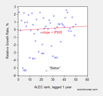
Figure 1: 2015 y/y growth rate of state relative to US coincident index, % versus 2014 ALEC rank, lower number is better. Red line is OLS regression line. Source: Philadelphia Fed, RSPS, author’s calculations.
Instead of the expected (at least by Arthur Laffer et al.) negative slope, OLS yields a postive (but statistically insignificant) slope coefficent. Omitting the outliers of WY, AK, ND, WV doesn’t change this basic result. The adjusted R2 is negative either way — there is essentially no explanatory power associated with the ALEC rankings.
The basic finding is unchanged if one considers GDP and/or different time horizons, as discussed in this post.
All this makes me wonder — exactly how much is ALEC paying Messrs. Laffer, Moore and Williams for this “analysis”?
Update, 4/14 11am Pacific: Because some readers (e.g., W.C. Varones) are unable and/or unwilling to click on cited references, I reprise this post from July 2015, which econometrically and fairly comprehensively assesses the usefulness of the ALEC sponsored RSPS rankings.
An Econometric Assessment of the World according to the American Legislative Exchange Council (ALEC)
For eight years, the American Legislative Exchange Council has been producing a ranking that purports to measure the competitiveness of individual states. From ALEC, Rich States, Poor States, 2015:
The Economic Outlook Ranking is a forecast based on a state’s current standing in 15 state policy variables. Each of these factors is influenced directly by state lawmakers through the legislative process. Generally speaking, states that spend less—especially on income transfer programs, and states that tax less—particularly on productive activities such as working or investing—experience higher growth rates than states that tax and spend more.
Hence I think it is reasonable to ask whether the ALEC-Laffer-Moore-Williams “economic outlook” ranking (hereafter “ALEC ranking”) actually has any predictive power, above and beyond other demographic and geographic indicators. This analysis follows up on a more ad hoc analysis in this post, and confirms conclusions arrived at in Fisher w/LeRoy and Mattera (2012). In addition, this analysis serves as a rejoinder to ALEC’s rebuttal asserting that critiques did not incorporate sufficient controls and allow for differing time horizons, to wit:
Moreover, rigorous statistical methods show that a higher economic outlook ranking in Rich States, Poor States does indeed correlate with a stronger state economy.
H/t Michael Hiltzik, who has done a tremendous job tracking the ALEC ranking. Let’s examine the available data.
Figure 1 depicts the one year growth in real Gross State Product and the ALEC ranking, lagged one year, for growth over the 2008-2014 period. Should the ALEC thesis be correct, one should see a negative sloped relationship.
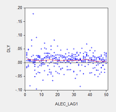
Figure 1: Real Gross State Product growth (log first difference) and lagged ALEC ranking for Economic Outlook. Nearest neighbor fit line (red), window = 0.3. Source: BEA and ALEC, Rich States, Poor States, 2015, and author’s calculations.
There is no obvious correlation between annual growth rates and the ALEC rankings. Note that lagging the ranking so that, for instance, the growth rate between 2013 and 2014 is related to the ALEC ranking in 2012 (instead of 2013) does not change the results much. (The ALEC 2013 ranking pertains to data reported in 2012, as far as I can tell). This outcome is unsurprising because the ALEC rankings are highly persistent. If one estimates a panel autoregressive model for the ALEC rankings, the AR coefficient is 0.95, and the adjusted R2 is 0.90.
Defenders of the ALEC rankings have argued that the rankings are aimed at predicting growth at a longer time horizon than annual. Given that the perspective of the RSPS methodology is supply-side, this argument is prima facie sensible. In order to accommodate that argument, I display in Figure 2 the data for three year (nonoverlapping) horizons (for 2014, and 2011).
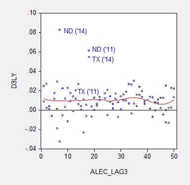
Figure 2: Nonoverlapping average three year real Gross State Product growth (log difference) and three year lagged ALEC ranking for Economic Outlook. Nearest neighbor fit line (red), window = 0.3. Source: BEA and ALEC, Rich States, Poor States, 2015, and author’s calculations.
Figure 3 provides analogous information, at the six year horizon (the maximum possible given the span of ALEC rankings).
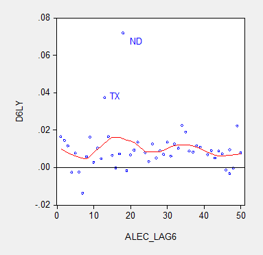
Figure 3: Average six year real Gross State Product growth (log difference) and six year lagged ALEC ranking for Economic Outlook. Nearest neighbor fit line (red), window = 0.3. Source: BEA and ALEC, Rich States, Poor States, 2015, and author’s calculations.
The nonparametric fitted lines indicate a slightly negative slope overall, suggesting some content to the argument that lower ranked states grow slower. In both Figures 2 and 3, North Dakota and Texas constitute outliers along the y-dimension. In order to discern how much these two observations drive the results, I omit them and replot in Figure 4.
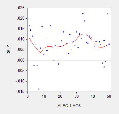
Figure 4: Average six year real Gross State Product growth (log difference) and six year lagged ALEC ranking for Economic Outlook, excluding North Dakota and Texas. Nearest neighbor fit line (red), window = 0.3. Source: BEA and ALEC, Rich States, Poor States, 2015, and author’s calculations.
No obvious pattern emerges from this last plot. In order to move beyond simple graphics, I now implement a series of regressions. First to a simple examination of the a bivariate relationship, encompassing the lower 48 states, one obtains at the annual frequency:
Δyi,t = -0.00003ALECi,t-1
Adj-R2 = -0.00, SER = 0.027, N=288. bold indicates significance at 10% msl, using heteroscedasticity and serial correlation corrected standard errors.
(I use the lower 48 as I do not have demographic and geographic data for the Alaska and Hawaii.)
Essentially, there is no explanatory power for the ALEC-Laffer indices in terms of year on year GSP real growth. Allowing for individual state-fixed effects, one obtains:
Δyi,t = 0.0004ALECi,t-1
Adj-R2 = -0.00, SER = 0.027, N=288. bold indicates significance at 11% msl, using heteroscedasticity and serial correlation corrected standard errors.
The coefficient is positive, indicating that lower ranked states, and hence states that have a less business friendly environment according the ALEC criterion, exhibit higher economic growth. The coefficient is borderline statistically significant. I would say that the use of state-level fixed effects is a fairly blunt way to account for state-specific factors. A better approach controls for state factors that economic theory suggests might be important for growth, such as geographic and demographic factors. Here we include log population density (LDENSITY, to account for urbanization), dryness (measured as inverse, WET), mildness of weather (MILD) and proximity to navigable waterways (DISTANCE); these four variables are defined such that positive coefficients are expected. These variables are time-invariant; hence one cannot estimate a fixed effects regression incorporating these variables. I also include log real price of oil (LRPOIL) to control for oil producing states, allowing the coefficient to vary across states.
Δyi,t = 0.0002ALECi,t-1-0.01LDENSITYi + 0.019WETi + 0.001MILDi + 0.0001DISTANCEi + LRPOILi,t
Adj-R2 = 0.36, SER = 0.021, N= 288. bold indicates significance at 10% msl, using heteroscedasticity and serial correlation corrected standard errors.
The ALEC ranking has no statistical significance, while a drier and more mild climate is associated with faster growth, with statistical significance. Proximity to navigable water is also a positive factor.
What if we estimate a comparable regression, looking at 6 year growth rates (but omitting oil prices which are the same for all states)? Then one obtains:
Δyi,t = -0.018 -0.0001ALECi,t-6 +0.001LDENSITYi – 0.0007WETi – 0.0003MILDi -0.00001DISTANCEi
Adj-R2 = -0.02, SER = 0.007, N= 48. bold indicates significance at 10% msl, using heteroscedasticity and serial correlation corrected standard errors.
Notice that the ALEC coefficient is not statistically significant. Thus far, the one case it has shown up as borderline significant, it goes the opposite of the ALEC-Laffer-Moore-Williams thesis.
Finally,Professor Ed (“no recession”) Lazear recently asserted that states with fast growing employment have low tax rates and right-to-work laws. He also argues that one needs to incorporate the depth of the drop in employment in 2008-09, in order to explain the growth in employment (so, a sort of version of the bounceback thesis he forwarded in the Economic Report of the President, 2009). I can’t find the working paper that provides the basis for his assertion, but I can estimate a comparable regression. In order to make the proposition testable, I examine 5 year growth rates in output, and refer to the ALEC rankings in 2009. I add the change in output from 2008 to 2009 (so TROUGHDEPTH takes on a value of -0.05 for observation i if output dropped 5% going into 2009).
Δyi,t = 0.065 -0.0010ALECi,t-5 +0.0046LDENSITYi + 0.0042WETi – 0.0014MILDi +0.00005DISTANCEi – 0.3413TROUGHDEPTHi
Adj-R2 = -0.04, SER = 0.037, N= 48. bold indicates significance at 10% msl, using heteroscedasticity corrected standard errors.
The ALEC variable does not exhibit statistical significance. Omitting ND and TX would not change this basic results. Moreover, the trough variable coefficient, while exhibiting the right sign, is not statistically significant.
Bottom line: The ALEC ranking, which purports to measure business-friendly policies, is not correlated with real GSP growth, either short term or medium term. This is true if one controls for additional variables.
I don’t think this necessarily means that policies such as right to work, or tax rates, and so forth do not have an impact on growth. For instance, Kolko, Neumark, and Cuellar Mejia, J.Reg.Stud. (2013) conclude that what’s important is “less spending on welfare and transfer payments; and more uniform and simpler corporate tax
structures.” Hence, the ALEC economic outlook ranking is, in my assessment, a manifestation of faith based economics.
Addendum: As Wisconsin has risen in ALEC rankings (33rd in 2008 to 17th in 2014), Wisconsin’s growth rate has declined relative to the US.

Figure 5: Wisconsin-US real growth differential (log first difference) and lagged ALEC ranking for Economic Outlook for Wisconsin (down is a “better” ranking). Light green shaded area pertains to GDP growth rates during the Walker era. Source: BEA and ALEC, Rich States, Poor States, 2015, and author’s calculations.
If it is not obvious, this is not the direction that ALEC-Laffer-Moore-Williams posit.
Note: Thanks to Professor Neumark, who kindly provided the data set used in his J.Reg.Stud. paper for use by my students in my PA819 statistics course (all students had to use his data set to analyze whether business conditions as measured by various indices (but not the ALEC ranking) influenced state level growth). The demographic and regional variables are drawn from that data set.
Using a single year during a massive energy bust and coastal real estate bubble to debunk the relationship between growth policies and growth.
Yep, sounds like ScienceTM to me!
W.C. Varones: Are you so lazy you can’t click on the link provided if you want different specifications? Or are you just remaining willfully ignorant, so you can write such rants.
But, given your previous comments, I suspect the latter is correct assessment…
If you want to provide substantive econometric/economic critique of the analysis contained in the more comprehensive analysis I linked to, I would welcome it.
Oil bust was larger this year and was basically unexpected. Surely you would have considered that before writing this rant……….
jeff: Yes, I had. If I drop 7 energy producing states, then the slope is slighly negative, statistically insignificant, with adjusted R-squared still negative. You will note that the uninformativeness of the ALEC ranking shows up with different indicators, different horizons, as I noted in this more comprehensive post (which I explicitly cited in the post).
If you want to provide a substantive econometric/economic critique of the analysis contained in the more comprehensive analysis I linked to, I would welcome it.
No matter how much lipstick you put on this pig it ain’t gonna fly!
These right wing “growth parameters” just doesn’t have much if any influence on growth. The easiest way to understand why is to look at the GDP formula its 70% consumption. The easiest way to increase consumption is to give more money to poor people (the consumer class). However, that kind of parameters will never be included in a right wing growth predictor index.
It’s not a 1:1 relationship, but here’s a map from Brookings showing influence of ALEC on state legislation/legislators.
http://www.brookings.edu/research/interactives/2013/map-alec-in-your-state
My guess is that Laugher’s charge was to show the afficacy of ALEC bills on state economies in order to keep the money flowing from donors.
Interesting that my 2 states are, according to ALEC, in the toilet, yet you can’t get a restaurant reservation on Friday night. And Burger King in the exurbs is paying 15 bucks and hour.
I know what “2 states” you’re talking about – Oz and Shangri-La.
Troll
Perhaps our economists can come up with two indices that can be applied to each state:
1 – money well spent
2 – money down the rabbit hole
The the states can spend more of 1 and less of 2 and we’ll all be prosperous.
Or will some seriously argue that all spending is good?
Bruce: could you define money well spent and money down the rabbet hole? Why does it make a difference to the economy in general?
I suspect “money down the rabbit hole” is code for money spent on “those people.”
If there is a significant output gap and interest rates are at the ZLB, then almost any government spending is money well spent. The cost/benefit threshold is pretty low in that case. As to money down a rabbit hole, a lot of DoD spending falls into that category…hey, you blow up what you just produced! I would also include tax subsidies for sports facilities as money down a rabbit hole.
The output gap represents people not working or working too little and therefore national income and aggregate demand are too low, because government is spending on people not working or working too little.
The U.S. has an global empire, which benefits the U.S. tremendously, and therefore needs to defend its empire, which includes national defense and deterrent.
Americans want sports stadiums and they’re willing to pay for the them. Sports stadiums also benefit local economies substantially. What Americans don’t want are more low income people.
The output gap represents people not working or working too little and therefore national income and aggregate demand are too low
Ah…so you’re a believer in Say’s Law. Too bad.
The U.S. has an global empire, which benefits the U.S. tremendously
And apparently you’re a running dog imperialist as well?
What Americans don’t want are more low income people.
Well, at least it’s an honest answer. No more riff-raff. No more of “those people.”
Americans want sports stadiums and they’re willing to pay for the them
No, upscale Americans want sports stadiums with exclusive skyboxes and want everyone else to pay for them. Why don’t more owners of sports teams self-finance all of these precious national assets. BTW, ask St. Louis folks how they feel about the Rams sticking them with a white elephant after the Rams bolted to LA.
It’s a lesson in incentives, and an explanation why the fiscal stimulus failed and deficit spending continues to fail.
Perhaps, you believe government spending and policies that immobilize or reduce resources, e.g. labor and capital, will mobilize or raise resources.
And, yes I want fewer low income people, unlike you.
So, we can build even more sports stadiums, convention centers, concert halls, etc..
So, you’re a believer the U.S. shouldn’t be a superpower. Well, your putting us on the right track.
If one estimates a panel autoregressive model for the ALEC rankings, the AR coefficient is 0.95
Sounds close to a panel unit root.
2slugbaits: Agreed, although it can’t literally be since rankings are bounded between 0 and 51.