A year ago, Jeff Frieden and I forecast (along with others) in Politico Magazine a boom in output. In light of today’s third release for 2014Q3 real GDP, clocking in at 5% SAAR [1], it’s reasonable to ask, are we there yet?
Figure 1 depicts the upward revision in GDP from advance to final, in the context of the last two years.
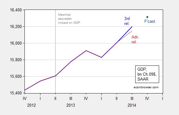
Figure 1: GDP, in billions of Ch.2009$, SAAR, 3rd release (bold blue), and advance (red). Macroeconomic Advisers tracking forecast as of 12/23 for 2014Q4 (dark blue square). Vertical dashed line at maximal estimated impact on GDP growth according to Macroeconomic Advisers (2/20/2014). Source: BEA 2014Q3 3rd and advance releases, and Macroeconomic Advisers.
Notice that there is a slowdown in 2013Q2 when Macroeconomic Advisers indicated the maximal impact on growth. (Notice that some observers have argued that since the growth impact was only estimated for two quarters, then the sequester had minimal impact. Of course, those with a familiarity with math recognize that a transient impact on growth has a long term impact on the level unless the impact on growth is offset.)
Where does a lot of the growth revision come from? The answer is in great part — services.
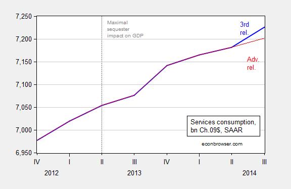
Figure 2: Services consumption, in billions of Ch.2009$, SAAR, 3rd release (bold blue), and advance (red). Vertical dashed line at maximal estimated impact on GDP growth according to Macroeconomic Advisers (2/20/2014). Source: BEA 2014Q3 3rd and advance releases.
The estimates of services consumption have been particularly problematic with the advent of ACA implementation (which by the way seems to be taking uninsured rates to new lows). But both health and non-health services consumption were revised upward.
One prediction we made was that investment would surge, given corporate profit levels and the decrease in policy uncertainty. This has come to pass only in part.
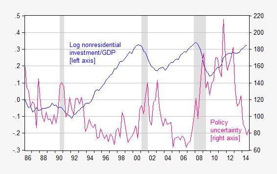
Figure 3: Log nonresidential fixed investment to GDP, both in billions of Ch.2009$, SAAR, 3rd release, rescaled to 1986Q1=0 (blue, left scale), and policy uncertainty index (pink, right scale). Policy uncertainty for 2014Q4 is through 12/23. Source: BEA 2014Q3 3rd release, and Baker, Bloom and Davis.
Notice that the investment series is business fixed investment, expressed as a log ratio to GDP. The series only has an interpretation in terms of cumulative differential growth rates since 1986Q1. (For a cautionary tale regarding the use of chain weighted quantities, see this post) By that metric, with the 0.8% upward revision of investment relative to advance, the 2014Q3 differential almost matches the differential of the last two peaks, with an acceleration in the last three quarters (as we predicted). That surge has occurred against a backdrop of reduced policy uncertainty.
That being said, the net ratio is probably lower since economic depreciation of capital has probably accelerated over the past decade as a higher proportion of investment is in shorter lived ICT capital and software.
Interestingly, radio silence on the release from the Joint Economic Committee (Republicans), who typically religiously send me critiques of the latest economic releases. Furman/CEA provides their assessment here.
A final observation: while growth is now proceeding more rapidly, with solid fundamentals in place for growth in 2015, it’s important to recall the CBO estimated output gap remains large, at 3.3% (log terms). Moreover, any number of international developments could still derail growth. As could another bout of fiscal brinksmanship (e.g., [2]).
Just to be difficult, note that the y/y growth in nominal GDP does not seem to be really accelerating even though the third quarter SAAR is very strong.
Some observations:
You data argues that against fiscal stimulus, as the sequester appears to have had only a two quarter impact. That’s why my analysis suggests as well. With the possible exception of the depths of a recession, the case for fiscal stimulus is not compelling.
Policy uncertainty is unrelated to investment. Since 2010, investment as a share of GDP has been rising steadily, regardless of the policy uncertainty.
Whether the output gap is 3.3% or 6% matters. At 4% GDP growth, a 3% gap will be closed by year end 2016, suggesting a possible recession for 2017, per JPM. If the gap is 6%, as you earlier stated, then the economy probably has running room through 2018. I think the 2007 trend line is the one to use.
Also, let’s keep an eye on government investment. I expect we’ll see some action there.
“suggesting a possible recession for 2017”
In what serious macro model can you predict a recession based on a projected closing of the output gap? This seems crazy.
The presumption would be that an economy at full output would begin to show stresses, eg, wage inflation, asset price bubbles, etc, which would ultimately trigger a recession.
Also, 2017 would be ten years since the last recession. The historical avg bus cycle in the US is five years.
But that’s asserted, not proven. It would be interesting to see a post on potential GDP and business cycles.
And by the way, Rowz, why don’t you do the work for a change?
The potential GDP data is at the IMF, here: http://www.imf.org/external/pubs/ft/weo/2014/02/weodata/index.aspx
US recessions are here: http://www.nber.org/cycles/cyclesmain.html
European recessions are here: http://www.cepr.org/content/euro-area-business-cycle-dating-committee
the sequester appears to have had only a two quarter impact.
Did you miss this part of Menzie’s post: …those with a familiarity with math recognize that a transient impact on growth has a long term impact on the level unless the impact on growth is offset.?
In any event, I don’t understand your point. Why should we accept any unnecessary reduction in growth if that reduction can be avoided? Your view seems to be that fiscal policy may be justified only if it will ameliorate a sharp fall in growth, but not a modest fall in growth. So in your view it would have been one thing if the impact of the sequester had been (say) ten quarters, but tolerating lower growth for only two quarters is just fine. What about three quarters? Or four quarters? You seem to have this view that fiscal policy is some highly toxic medicine that is only to be used in extremis. I don’t get that. To me it’s just nuts. Why would anyone deliberately choose an unnecessary and entirely avoidable austerity policy that has no upside simply because you think the downside won’t be too bad?
It seems to me, Slugs, that the notion of potential GDP in itself suggests constraints on the use of stimulus. If you believe in the concept of potential GDP, then that also seems to imply some ‘natural’ rate of GDP growth, which by definition can’t be altered very much. If you reject that notion, then potential GDP is bouncing around as a function of GDP, and I’m not sure potential GDP as a concept has much value, because estimating the gap itself becomes highly problematic.
Therefore, it seems to me from the graph above that the sequester has a two quarter effect, after which GDP returns to trend. If I further believe there is some natural rate of growth which determines long-run GDP, then the effect of the sequester fades by definition, ie, we cannot sustainably raise GDP growth above its natural long-term pace once the output gap is closed. Therefore, your policy space is limited to the output gap with the stimulus minus the output gap without the stimulus. That’s not 35% of GDP–which is how much our debt has increased. If it were, the debt should have paid for itself, which obviously it has not. (This is the mirror argument to the supply-side tax cuts raising revenues, no?)
In any event, the very short effect of the sequester suggests that deficit spending does not, in fact, increase long-term growth. A sustainable economy occurs when a willing seller can make things at an acceptable profit which a willing buyer will purchase. If the government gives money to an individual who cannot create the value they themselves consume, then the purchasing power will disappear when the government funding does. In other words, government spending does not create a sustainable economy by itself. And this shows in the GDP data. As you can see in this post, there is simply no relationship between deficits and GDP growth across the OECD. http://www.prienga.com/blog/2014/11/28/deficit-spending-and-gdp-growth
1. Turns out Obamacare didn’t tank the economy and …
2. The policy uncertainty many claimed was THE thing holding back the economy went away when Obamacare started and has continued to drop.
I’m not crowing or arguing, just observing. I think it’s fine to argue that “this or that will be harmful” but it’s just as important to say “oops”.
It was fascinating to reread the Politico piece and to see how so many are bluntly wrong. I never expect more but it’s interesting to see how off these were in one year.
The comments are pretty good too. like this one:
“Mark Woodworth, Ph.D. • a year ago
Read zerohedge to get the truth”
Can you get a refund on a Ph.D.?
Our politicians in Washington could’ve been more effective, and less counterproductive, getting the economy on track, and assisting the Federal Reserve.
Massive idle resources for this long is completely unnecessary.
Anyway, here are some charts:
http://www.advisorperspectives.com/dshort/
I just completed James Grant’s book THE FORGOTTEN DEPRESSION about the depression of 1920-21. He points out the difference between this depression and the Great Depression that began in 1929. Most important was that in 1920-21 the government, the financial press, and the people not only did not stop the decline in prices and waged, they celebrated them. They knew that the prices of the factors of production had risen beyond the level the free market could sustain and that the solution was to allow costs to quickly return to normal – the political slogan of the time. The currency remained steady and the gold standard was allowed to work (it was not subverted until the Genoa Conference in 1922 and did not impact the US until 1927 when Strong began to prop up the pound). The decline was over in 18 months and the recovery was one of the fastest and largest in history.
On the other hand in November of 1929, Herbert Hoover called in all the major business leaders and had them pledge not to lower wages. Only Treasury Secretary Mellon called for price declines and “liquidation” but he had no support and was ridiculed. Hoover had bought into the socialist propaganda of the time and he rejected Mellon’s plan for recovery (that worked in 1920-21). Hoover got the answer backward and when it didn’t work he began to push government spending. The value of the currency was not stable. FDR ran his 1932 campaign much like the political campaign of a return to normalcy, but once in the Presidency he did not govern as he campaigned adopting virtually all of Hoover’s policies. The result was stagnation and the longest depression in US history that did not recover until after WWII after wages and prices had fallen to pre-1929 levels.
So what happened at the start of the Great Recession? Was it the ideas of Mellon or of Hoover that ruled the day? Prices of real estate crashed and foreclosures exploded. The cost of capital declined in some sectors but was held artificially high in others. Minimum wages were raised three times, unemployment insurance was increased to the greatest level in US history and created the same situation as in the UK during the 1920. Today the work force is lower than when the crash began and real wages have been slowly falling. The factors of production have fallen despite the attempts to prevent it. With the fall in wages and cost of capital along with a stabilization in the currency and the decline in government spending (thank the Republicans) the economy is set for recovery. The wild care in al of this is how destructive the ACA will be as it becomes fully implemented. It has been a huge drag on the economy and the largest changes to the health care insurance of businesses is still being pushed out. Once the ACA destroys business health care plans there is no way to know the impact because it continues to constantly change and we do not know how congress will impact the damage.
It is commendable that some of the economists recognize that declining prices have contributed to the conditions for recovery. It is sad that when they “stressed that recovery would be long and slow” they did not carry this analysis deeper. Rapid recovery could have come in 18 months, or even less. Hopefully the Republicans will honor the wishes of the voters and not be seduced by the destructive policies of the Progressive left.
Ricardo, the 1920-21 recession/deflationary depression was a Long Wave Peak recession as in 1980-82, 1860s, 1810s, and late 18th century, which were periods associated with peak demographic effects, war, or energy and materials.
Economists have been taught for a generation or two now that the Long (Kondratieff/Kondratiev) Wave does not exist, but the response by central banks and gov’ts since 2008, and before that in Japan since the 1990s, is clear evidence of their leaning against, and desperately attempting to postpone or prevent, the debt-deflationary forces associated with the Schumpeterian Long Wave depression or debt-deflationary regime of the Long Wave Trough, as in the 1790s, 1830s-40s, 1890s, 1930s-40s, and Japan since 1998.
Were the Long Wave to remain in force, peak Boomer demographics (and now in China and the Asian city-states), debt to wages and GDP, equity valuations to profits and GDP, and labor’s share of GDP all combine to suggest that the debt-deflationary regime of the Long Wave to date will persist into the end of the decade to the early 2020s, including decelerating real GDP per capita and CPI, as well as the 10-year US Treasury yield eventually matching those of Japan and parts of the EZ at 1% or lower.
Although the likes of Larry Summers surely knows this but cannot say so publicly, his use of the term “secular stagnation” is another way of saying the Schumpeterian Long Wave Trough depression or “slow-motion depression” as I also refer to it, given hyper-interventionist central bank and gov’t policies and gov’t, health care, education, and debt service combining for well over 50% equivalent of GDP resulting in the “hyper-financialization” of the US economy.
The “hyper-financialization” of the economy is manifested primarily by the fact that total annual net flows to the US financial sector and the top 0.1-1% from rentier (interest, dividends, capital gains, pass-through income from real estate, and fees received from managing financial assets) flows equal or exceed the annual growth of nominal value-added output of the US economy. In other words, all nominal GDP is currently pledged to the rentier claims of the US financial sector (and financialized sectors, including insurance, education, and health care) and the top 0.1-1% indefinitely hereafter.
Therefore, if one receives one’s income, wealth, and socioeconomic status from the rentier-parasitic, hyper-financialized sectors, conditions have never been better, and the suggestion that the US is in a “slow-motion depression” is absurd.
However, for the bottom 90%+ of households who rely upon earned income from wages and salaries for subsistence, including the self-employed, or from transfer payments received from taxing wages and salaries, it’s anything but the best of times.
Finally, the larger the financial bubbles are inflated as a share of wages, profits, GDP, and gov’t receipts, the larger and more persistent the rentier claims against same by the owners and direct and indirect beneficiaries of the rentier claims, and thus the slower real GDP/final sales per capita will be indefinitely hereafter.
The hyper-financialization of the US economy has permitted an unprecedented hoarding of financial assets at no velocity and increasing claims to the bottom 90-99% by the top 0.01-0.1%.
Historically, these conditions have presaged financial and currency crises; debt/asset deflation and private and public debt defaults; privation for the working-class masses; social instability; an existential threat to socioeconomic status and well-being of the buffer caste between the elite top 0.1-1% and the masses, i.e., today’s professional middle class 9% below the top 1%; loss of confidence in financial, economic, and political institutions; violent reaction by gov’ts against the masses; war and mass destruction at increasing scale of property and human life; and r-evolution.
Here is someone to argue with about 1920-21
http://econospeak.blogspot.com/2014/12/are-keynesians-desperate-about-1921.html
BTW that was the years my dad and mom, newly married, graduated from college and could not find jobs as teachers. They had to come back to California to live with my grand dad for a while.
“The wild care in al of this is how destructive the ACA will be as it becomes fully implemented. It has been a huge drag on the economy and the largest changes to the health care insurance of businesses is still being pushed out. Once the ACA destroys business health care plans there is no way to know the impact because it continues to constantly change and we do not know how congress will impact the damage.”
where do you come up with this garbage? show me this “huge drag” outside the fantasyland of faux news.
Auto sales and the oil and gas boom/bubble have contributed disproportionately to the growth of industrial production (IP), employment, and thus overall growth of (un)economic activity since 2010-11.
Auto sales have likely peaked, as subprime auto loans have accounted for one-third of sales and delinquencies have risen since early 2014. The crash in the price of oil will likely reduce demand for EVs.
Oil and gas extraction and energy-related transport has skewed IP higher than otherwise would have occurred. The crash in the price of oil will hit oil and gas extraction and energy-related transport and thus drag on IP in H1 2015.
The decline in the price of oil YoY of 40% or more has occurred coincident with recessions, bear markets, and a dramatic deceleration or deflation in prices (on the gold or gold exchange standard for most of the time, however), including 2008-09, going back to the Civil War, with the exception of 1986 (the onset of US deindustrialization, financialization, and debt to wages and GDP increasing an order of exponential magnitude into 2007-08).
Housing is rolling over again, with high-multiplier housing overall now a diminishing influence on US (un)economic activity compared to the post-WW II period through 2006-07. This is likely to be a secular (permanent?) trend as the composition of household spending experiences a once-in-history shift from high-multiplier spending for housing, autos, and child rearing to low-multiplier spending for house maintenance, property taxes, utilities, food at home, insurance, and out-of-pocket costs of medical services and medications. This will result in the ongoing deceleration of the 10-year change or real final sales per capita below 1%, i.e., “secular stagnation” or a “slow-motion depression” as in Japan since the 1990s.
Jobless claims to payrolls are at the lows of the peaks in 2000 and 2006-07 (when the U rate bottomed) with little or no growth in the labor force and a surge recently in the number of workers with multiple jobs, including those with full-time jobs and at least one part-time job. There is evidence of labor hoarding, which is characteristic of cyclical peaks.
US total gov’t spending (including war spending), private “health care” and “education” spending, household and business debt service, and oil consumption to GDP combine for an equivalent of 56% of GDP. The US economy cannot grow unless there is growth of gov’t spending for war, food stamps, and Obamacare, illness, too many high school students obtaining student loans they can’t afford to pay back, and firms and households take on more debt as a share of GDP. However, that these sectors account for more than 50% equivalent of GDP, the growth of these sectors exert a drag on the remaining 46% of the economy.
Once autos, oil and gas extraction, and energy-related transport rolls over, there are no other sectors to take up the cyclical slack in order to sustain growth, and “health care” insurance and out-of-pocket costs will become an increasing constraint on US (un)economic activity hereafter. Gov’t spending and deficits as a share of GDP will likely increase again for the cycle beginning in 2015.
Finally, the stock market is exhibiting an exceptionally rare precedent of coincident conditions occurring:
10-year average P/E above 20.
Market capitalization at or above 100% of GDP.
Record non-financial corporate and margin debt to GDP.
Record profits to GDP.
Hindenburg Omen.
Weekly and monthly Tom DeMark sell signals.
A log-periodic, super-exponential blow-off having occurred since 2012.
Only one other period in the US since the 1920s exhibited these same conditions simultaneously: 1929-30.
The top in 1987 occurred coincident with four of the seven phenomena.
That it is likely that the fiscal deficit to GDP will increase in 2015 with decelerating GDP below this year’s ~2.5% and CPI to 1% or below, the Fed will not raise the bank reserve rate and will probably resume QEternity at ZIRP at some point in 2015.
Is that really “Log nonresidential fixed investment to GDP” = log[NRFI/GDP]
or is it the log of the ratio of the annual percentage changes = log{[delta(NRFI)/NRFI_o]/[delta(GDP)/GDP_o]}
?
tew: Let X[t] be nonresidential investment at time t, X[0] at base period, Y[t] GDP at time t, Y[0] at base period (all in chained 2009$). Then I have plotted log(X[t]/X[0])-log(Y[t]/Y[0]).
Thank you for your reply. The calculation is the same as the latter one I’d written (*), except I was wrong about it being in terms of annual change. It’s now clear to me why doing it as a fraction of a base year is useful.
* log(A/B) = log(A) – log(B)
It seems, there are people who confuse prices and wages.
Lower prices can clear the market and increase production.
However, when there are no customers, a business won’t spend on inventories, hire workers, and expand.
A large tax cut and an increase in government expenditures can create customers.
An example of increased government spending to clear the market (from my statement in early 2009):
Instead of loans for the auto industry, the government should buy autos and give them away to government employees (e.g. a fringe benefit). So, automakers can continue to produce, instead of shutting down their plants for a month. Auto producers should take advantage of lower costs for raw materials and energy, and generate a multiplier effect in related industries.
http://www.markiteconomics.com/Survey/PressRelease.mvc/0539167ca8dd4b0088095675a7a3af71
http://www.markiteconomics.com/Survey/PressRelease.mvc/201ab60916734bff84245deb22eb39eb
http://www.markiteconomics.com/Survey/PressRelease.mvc/9bf921c24e49468ebcb1a1c26a9183d5
http://www.markiteconomics.com/Survey/PressRelease.mvc/5ae226e01c7044b5b409e82e0c306318
http://www.markiteconomics.com/Survey/PressRelease.mvc/69a0d2d7ecd640b6be58e210bc9f3a84
http://www.markiteconomics.com/Survey/PressRelease.mvc/81cd7459dab241dbbdde5e87c3dd1ae6
65-70% of world GDP in aggregate is at the historical stall speed or slower. This is occurring within the cyclical trend of real final sales of ~2% vs. 3.3% long term, and ~1% per capita vs. 2.1% long term.
The cyclical trend is occurring within the secular deceleration of real final sales from 2.4% since 2007 to 1.1% and at 0.4% per capita, and 1.8% since 2000 and at ~1% per capita.
So, the range for the ongoing secular trend rate of real final sales is 1.1-1.8% and 0.4-1% per capita, which is the the same trend as Japan since 1990 and 1990 and the US from 1929 to before WW II, as well as during the 1890s and 1830s-40s, i.e., debt-deflationary regime of the Long Wave Trough or Schumpeterian depression. Demographics, asset valuations, and debt to wages and GDP imply that this trend, or slower, will persist into the early 2020s.
This secular trend expectation is supported by the Chicago Fed paper on demographics-induced decline in labor force participation and payroll growth hereafter:
file:///home/bruce/Downloads/4q2014-part1-aaronson-etal-pdf%20(1).pdf
The slowing of labor force growth and decelerating labor productivity (owing to the ongoing decline in labor’s share of GDP and the Marxian falling rate of real growth of after-tax profits from 5.1% since 1997 to 2.4% since 1996) to below 1% since 2010 and 1.4% since 2007 from ~2% in 2000 similarly supports the ongoing trend of real GDP/final sales and per capita.
Thus, the trend of 0.4-1% real final sales per capita is as good as it gets given the drag effects from (1) debt to wages and GDP; (2) falling labor force participation and little or no growth of the labor force; (3) a record low for labor’s share of GDP; (4) decelerating labor productivity; and (5) a Marxian decline in the real rate of growth of profits, particularly for non-financial after-tax profits having decelerated from 4.2% since 1996 to 1.1% since 2006.
A once-in-history acceleration in the automation of services labor hereafter from the growth of use of smarts systems, Big Data analytics, biometrics, bioinformatics, nano-electronic sensors, quantum computing, etc., will exert a further constraint on labor’s share of GDP, employment, wages, and purchasing power of the bottom 90%+, and thus reinforce the structural drag on overall growth, including growth of gov’t receipts and the resulting resumption of the increase in the fiscal deficit as a share of GDP.
The world is turning Japanese, but we can’t be permitted to act as though we know it or believe it, as it implies that Japan-like policies the Fed and ECB are engaged in will yield the same results that Japan has achieved for the past 16-24 years.
Corrections: “1990 and 1998” instead of “1990 and 1990”, and “smart systems” instead of “smarts systems”.