One important factor in the growth prospects for the US economy is the trajectory of the dollar. [1] If the dollar stabilizes at March levels, US economic growth might rebound. On the other hand, continued appreciation bodes ill. Based on history over the floating rate era, the expected duration of an appreciation is about 5 years (depreciations about 2 years). The current surge in the dollar has only been going on for only slightly over half a year, although when dated from the trough of 2011Q2, it’s been going on just a bit over 4 years. Either way, by this metric, it appears that there is still some additional way to go before the dollar peaks.
Figure 1 shows the evolution of the real value of the dollar against a broad basket of currencies; description of the construction of such indices is detailed in this paper.
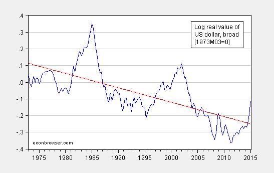
Figure 1: Log real value of US dollar against broad basket of currencies (blue) and linear trend (red). Source: Federal Reserve Board and author’s calculations.
While it is common to characterize exchange rates as a random walk, for real rates, this characterization is not completely apt. One can reject a unit root (allowing for a trend) at marginal levels, using the Elliott-Rothenberg-Stock unit root test. The trend obtained using OLS indicates a trend depreciation at about 0.9% per year.
More interestingly, an inspection of Figure 1 suggests that there are long swings in the dollar’s value. This observation is not new, and was first made 25 years ago by Engel and Hamilton (AER, 1990). The fact that when the dollar appreciates, it continues to appreciate is suggestive that the dollar’s current ascent is not yet over.
Long Swings Re-evaluated
In order to make an updated assessment, I take data over the 1973-2014 period, and estimate a Markov Switching model. The dependent variable is the year-on-year change in the log value of the dollar, sampled in the fourth quarter of each year.
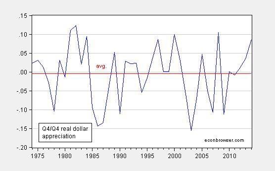
Figure 2: Q4/Q4 change in log real value of US dollar against broad basket of currencies (blue) and average over 1974-2014 (red). Source: Federal Reserve Board and author’s calculations.
A common coefficient is placed on a dummy variable for the financial crisis, taking on a value of unity in 2008. Assuming a constant variance over two regimes, I estimate an upswing regime with real appreciation of 3% per annum and downswing regime with real depreciation of 10% per annum. The financial crisis appreciated the dollar by 20%, according to the estimates (see here).
The probability of staying in regime 1 (appreciation) conditional on being in regime 1 is 81%; the probability of transitioning to regime 2 (depreciation) from regime 1 is 19%. The probability of staying in regime 2 conditional on being in regime 2 is 44%; in contrast, the probability of transitioning into regime 1 when in regime 2 is 56%.
The smoothed regime probabilities are presented in Figure 3:
Figure 3: Smoothed regime probabilities for regime 1 (appreciation) and regime 2 (depreciation) estimated on annual data, 1974-2014. Source: Federal Reserve Board and author’s calculations.
Hence, as of 2014, the US dollar was likely in appreciation regime. Using semi-annual data, one obtains similar implications (the dollar is an appreciation regime), but the expected duration is somewhat shorter – a bit less than three years for an appreciation regime, and a year and a half for depreciation regime. In this case, the dollar appreciation is already a bit long in the tooth. The ambiguity is not unexpected; Engel (1994) found that it was hard to exploit the long swing characteristic in such a way as to outperform a random walk.
I tend to favor the interpretation associated with the one year changes in the real rate given that this matches with the interpretation of long swings seen in Figure 1.
A Threshold View
Another way of interpreting the data exhibited in Figure 1 is to think of there being thresholds around (possibly trending) parity in the real exchange rate (e.g., the red line). The thresholds could be sharp (e.g., O’Connell, JIMF, 1998), or smooth (e.g, Taylor, Sarno, Peel, IER, 2001, among many others). Close to parity (in this interpretation, close to the red line), reversion to trend would be very slow, and far away, quite rapid.
O’Connell (1998) sets the threshold at 0.12 for the US bilateral (CPI-deflated) exchange rate against other industrial countries, estimated over 1979-95. In the smooth threshold approach, the pace of reversion is monotonically faster the farther away from parity. In Taylor, et al. estimates, a 40% shock has a half-life of a deviation of less than a year; a small shock has a half life of over three years (for two key bilateral US real rates, over the 1973-1996 period.
This idea of thresholds has made it into the practitioner literature. Figure 2 displays the Deutsche Bank (March 30, 2015 [not online]) take on the nominal rate; fair value is defined by purchasing power parity (relative price levels).
Figure 2 from Chadha, Thatte, Tierney, “Global Asset Allocation: The Dollar fast cycle,” World Outlook, March 30, 2015 [not online].
Hence, this graph is the nominal analogue to Figure 1 (except the currency baskets are different). The +/- 20% bands are their interpretation of the relevant thresholds. DB assesses the dollar at 10% above parity as of March 2015. Using the estimated real dollar trend (which assumes cointegration between the exchange rate and relative prices with unit coefficient), my calculation in Figure 1 implies the dollar is 14% overvalued, and thus yet to breach the threshold.
Summing Up
By the long-swing metric, there seems to be some more appreciation in store. The same is true using a threshold approach. However, these conclusions are based upon historical patterns, for which there are not many independent observations – two and a half dollar cycles essentially. In addition, there is no guarantee that these patterns will persist. From Chadha, Thatte, and Tierney:
The US dollar has risen since last summer against the major currencies at the fastest paces on record, up 21%. Compared to a typical dollar cycle that spans from 20% below to 20% above fair value over 6-7 years, we have seen 3 years of appreciation packed into 9 months. Current levels put the dollar 10% above fair value and 3/4 of the way through a typical cycle.
In other words, the sheer rapidity of the dollar surge may mean a different outcome this time around, and the dollar appreciation might end sooner than suggested by the previous discussion. That would remove some of the drag on economic growth [1]
For more, on other “fair value” or “equilibrium” approaches, see [2], [3], and [4].
Since the tired old lie of the ‘pay gap’ doesn’t seem to die…
Professor Mark J. Perry (an economics professor of considerably higher stature than Menzie Chinn) draws attention to ‘Equal Occupational Fatality Day’.
http://www.aei.org/publication/equal-pay-day-this-year-is-april-14-the-next-equal-occupational-fatality-day-will-occur-on-july-29-2027/
Men are 93% of all workplace deaths.
Yet another example of how knowledge of economics is mutually exclusive with a belief in contemporary ‘feminist’ dogma.
you could close the gap by enforcing osha safety standards in the high risk jobs employed by men.
Menzie,
I was very interested in this post before I read it, but I was very disappointed. You could have based your analysis on sun spots, fungus on tree trunks, or astrological charts. But all of these (including your analysis) assumes away the primary responsibility of the FED – maintaining a stable currency. If we take your analysis based on uncontrolable trends as fact, the huge question is then why do we even have a FED? If monetary stability is beyond the control of the FED then why do we even have a FED?
I totally disagree with this. I do believe that the FED could maintain the stability of the dollar. The wide fluctuation illustrated in your graphs reveal the serious failures of the FED to perform its primary responsibility. As a matter of fact your graphs are the biggest indictment of the FED I have seen in a long time.
The FED has a duel mandate “to promote effectively the goals of 1) maximum employment, 2) stable prices and moderate long-term interest rates.” It deserves a huge F minus on its report card on both.
It seems, the U.S. dollar to a broad basket of currencies and the U.S. dollar to the euro is highly correlated.
‘The fact that when the dollar appreciates, it continues to appreciate is suggestive that the dollar’s current ascent is not yet over.’
And that advice is worth every dollar we’re paying for it!
Just when I think Menzie couldn’t be any more ridiculous ….
Patrick R. Sullivan: Thank you for your tremendously insightful comment, typical of the commentary we have come to expect from you. After all, you have stated unequivocally:
And this statement is wrong, like pretty much everything else you write down.
It would be useful for you to sometime acquaint yourself with the large empirical literature on real exchange rate behavior (actually, your acquaintance with just plain ol’ facts would be an advance!). In point of fact, the belief in a random walk real exchange rate is most closely associated with the neoclassical school of open economy macro, in particular those that believed in intertemporal optimization, flexible prices, and a large role for technology shocks. So, if you are dismissive of the random walk interpretation, we are in agreement! (I’ll bet that’s a surprise to you…)
Think the world’s central banks might have something to say about that?
Re: Oil Prices
Following is Steven Kopits (January, 2015) chart showing his outlook for global liquids production (crude, condensate, NGL and biofuels) less liquids consumption, and Steven has been on record I believe as predicting an oil price rebound (the Prienga curve is Steven’s outlook):
http://i1095.photobucket.com/albums/i475/westexas/Supply%20Minus%20Demand_zpswyvmrvkw.png
Note that the initial short term (three month) and longer term (26 month) recovery in monthly Brent prices during the 2008/2009 oil price decline was 43%/year, relative to the December, 2008 monthly oil price low (when Brent averaged $40). Monthly Brent prices rose at 43%/year from 12/08 to 2/11, when monthly Brent prices once again exceeded $100 per barrel.
The (so far at least) low point for monthly Brent prices for the current decline was January, 2015, when Brent averaged $48. Brent is currently at $58. If Brent averages $60 for April, 2015, the initial short term annualized rate of increase in monthly Brent prices will have been about 90%/year.
FT update on Greece:
Greece prepares for debt default if talks with creditors fail
http://www.ft.com/intl/cms/s/0/c5964f9c-e1ef-11e4-bb7f-00144feab7de.html#axzz3XIFE9hww
Indeed, imposing some empirical model on a highly regulated animal like the value of fiat currency seems quite odd. Are you predicting the Fed reaction functions here? Plus, with currencies, of course, there are the domestic regulators (the Fed) and the foreign regulators (ECB, Japan, China), all reacting to events. Seems like a political model of fiat currency values is more appropriate than an empirical model.
From forecasters to innovators – Trillion Dollar Economists: How Economists and Their Ideas have Transformed Business (http://eu.wiley.com/WileyCDA/WileyTitle/productCd-1118781805.html)
I would rather see an analysis based on capital flows and interest rates. It seems clear that what happened was the Fed created a dollar carry trade that is now being reversed. This would have happened, even if the Fed and ECB had not switched places in regards to QE practices. I think the reason for the especially rapid recent dollar rise is that the reversal of the dollar carry trade is being reinforced by monetary policies abroad (ECB and Japan). I came to the same conclusions you did (dollar appreciation will end, but not just yet), but from a different perspective. I had been long on the dollar until just recently. Now, I’m waiting to short the dollar. For those engaged in such activities, figure 2 (the last one) is much more interesting than your other figures.
menzie,
thanks for this interesting post.
I was trying to replicate your results on the markov switching model
no problem on the mechanics of the model but it seems I am not able to get the real dollar data right.
Did you use the real US dollar Broad index of the FED (http://www.federalreserve.gov/releases/h10/summary/indexbc_m.htm) ?
then simply a december/december y-1 percentage change (or ln differential), or an average of the Q4.
I tried both but the change is not what is shown in your post
rafiminos: I used Q4/Q4 log difference, at annual frequency — so latter. The command was switchreg(type=markov) dlr_y c @pv fincrisis , where dlr_y is Q4/Q4 log difference of real broad exchange rate. fincrisis is dummy variable taking on a value of 1 in 2008. The variances in the two regimes are assumed the same (this is critical). See output here.
To my pleasant surprise I think I agree with Professor Chinn.
As anyone who has traded currencies will tell you – if can’t predict the future it is wise to assume serial correlation in S-T currency movements. As to the comments about the Fed controlling the S-T level of the $, currency markets are the largest and most liquid in the world. Central banks can nudge currencies but often with perverse consequences.
And anyone who aspires to trade currencies S-T using some more or less rational belief about knowing the ‘right’ exchange rate – unless you are working in the trading room of JP Morgan, Barclays, etc. – you are the one born every minute. Good luck.
A fellow trader – but with a different take. I trade very long term based on my perception of the ‘right’ exchange rate (basically, PPP, when the divergence can be explained, at least to my mind, by unusual capital flows, whether from monetary response to cyclical changes in the economy or from some unusual geopolitical event). Often, I start too early and increase my exposure as the actual exchange rate continues to diverge from my perceived ‘right’ rate. So far, I have always won (though I sometimes have had to wait a long time), but I have often wondered if a better strategy would be to simply use the serial nature of exchange rate movements. For one thing, I wouldn’t have to wait for opportunities. I average about 10% – 15% per year on exposure (not capital invested , i.e. the margin requirement).
I think losers are easy enough to explain – the odds are much better than Vegas (trading costs are minimal) and the game can’t be fixed. Many participants are there just for the utility from gambling. I admit I enjoy tuning in to Bloomberg every morning.